Modeling stochastic systems with Observable Operator Models
Motivation and basic idea
Stochastic time series data have “memory”, that is, what will happen in the future is influenced by what has happened in the past. The classical machine learning models of such systems are Hidden Markov Models (HMMs) for uncontrolled processes (like speech, biosignals, financial indices) and their extension to controlled processes (like robot motor control or intelligent decision making), called partially observable Markov decision processes (POMDPs). Deep learning research has recently led to variants of HMMs and POMDPs which include neural network components. All these models are trained by iterative local optimization methods which are computationally expensive and may get trapped in local (sub-)optima.
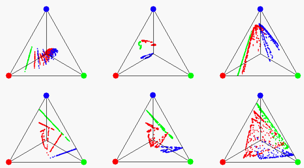
Observable operator models (OOMs) and their extension to controlled processes, input-output observable operator models (IO-OOMs) are alternatives to HMMs and POMDPs, respectively, introduced by Herbert Jaeger in 1997. OOMs, although superficially similar to HMMs, spring from a very different mathematical idea. While usually stochastic processes are mathematically modeled as a trajectory in some state space - where locations in that space correspond to the physical states of the modeled system -, OOMs operate on states which encode probability distributions over future continuations of a process. The state update operators are identified with the observables, hence the name, “observable operator models”.
Mathematical and algorithmical properties, impact
OOMs (and similarly, IO-OOMs) have intriguing properties:
- They generalize HMMs (POMDPs, respectively) in the sense that finite-dimensional OOMs can model a properly larger class of processes than finite-dimensional HMMs.
- Single-step, global and asymptotically correct learning algorithms for OOMs exist, in contrast to the known learning procedures for HMMs, which are iterative, local, and not asymptotically correct.
- The core idea of OOMs (states = future process distribution; update operators: linear) can be applied to any stochastic system, rendering OOM theory a general theory of stochastic processes which embeds stochastic process theory within linear algebra.
Due to its generality and transparency, OOM theory was adopted in a diversity of disciplines:
- in a re-formulation of basic ergodic theory, yielding, among other, very short proofs for classical theorems which before required long proofs (PhD thesis of Alexander Schönhuth 2007 (in German), co-supervisor H. Jaeger);
- in a re-formulation of parts of quantum mechanics (Ulrich Faigle and Alexander Schönhuth, see for example a 2015 arXiv paper);
- in machine learning, where OOMs triggered the development of predictive state representations (PSRs), now an active subfield in reinforcement learning (classic early paper);
- in chemical physics, where fundamental mathematical properties of OOMs were exploited to predict asymptotic properties of molecular reaction processes (group of Frank Noé, FU Berlin 2017 sample paper).
Current limitations and ongoing research
There are two reasons why OOMs and IO-OOMs have so far been put to only limited practical exploits in machine learning:
- The currently available learning algorithms are confined to symbolic, discrete-time processes. But the majority of technical applications demands models of continuous-valued processes.
- For maximizing statistical efficiency, the learning algorithms include nontrivial spectral compression steps whose mathematics and algorithmics are challenging. Robust “out-of-the-box” statistically optimal algorithms are not yet available.
The first issue requires the investigation of suitable projections of continuous value spaces to finite-dimensional probability vectors. While proof-of-principle methods have been demonstrated (outlined in the OOM tutorial indicated below), this line of work is waiting for an energetic researcher to take it on.
The second issue has been almost solved in the PhD project of Michael Thon.
References and code
Tutorial
Comprehensive OOM tutorial slides
References
- First report: H. Jaeger (1997), Observable Operator Models and Conditioned Continuation Representations. Technical report, Arbeitspapiere der GMD 1043, GMD, St. Augustin 1997 (38 pp) (pdf)
- Standard early reference: H. Jaeger (2000), Observable operator models for discrete stochastic time series. Neural Computation 12(6), 2000, 1371-1398 (pdf)
- Latest progress in spectral learning of OOMs and IO-OOMs, plus a method to deal with missing values: M. Thon (2017), Spectral Learning of Sequential Systems. PhD thesis, 167 pp. (pdf)
Code
- tom, a C++/Python toolkit for observable operator modeling, developed by Michael Thon